Tutorial: Simulation of conventional GC

In this post I want to give a tutorial on how to use the notebook simulation_conventional_GC.jl to run simulations for a simple GC system. Installing the needed software and how to start a notebook was shown in the previous tutorial. The notebook can be found under this URL.

The presented notebook can be used to simulate separation of mixes of substances on a simple GC using one column with a selected stationary phase and a temperature program for the whole column. No separately heated zones of the column exist. Most one-dimensional GC systems can be approximated with this simulation. In most cases separately heated zones, like in the injector and transfer line to the detector, can be neglected in comparison to the much longer section of the column in the GC oven.

In the following I will go through the notebook section by section and explain, what settings can be made, what the results are and how to export the results.

Header

In the header the needed packages are load. This can take some time, especially loading for the first time after installing Julia. The name of the notebook is indicated here. The unhidden code looks like this if the packages are successfully loaded: 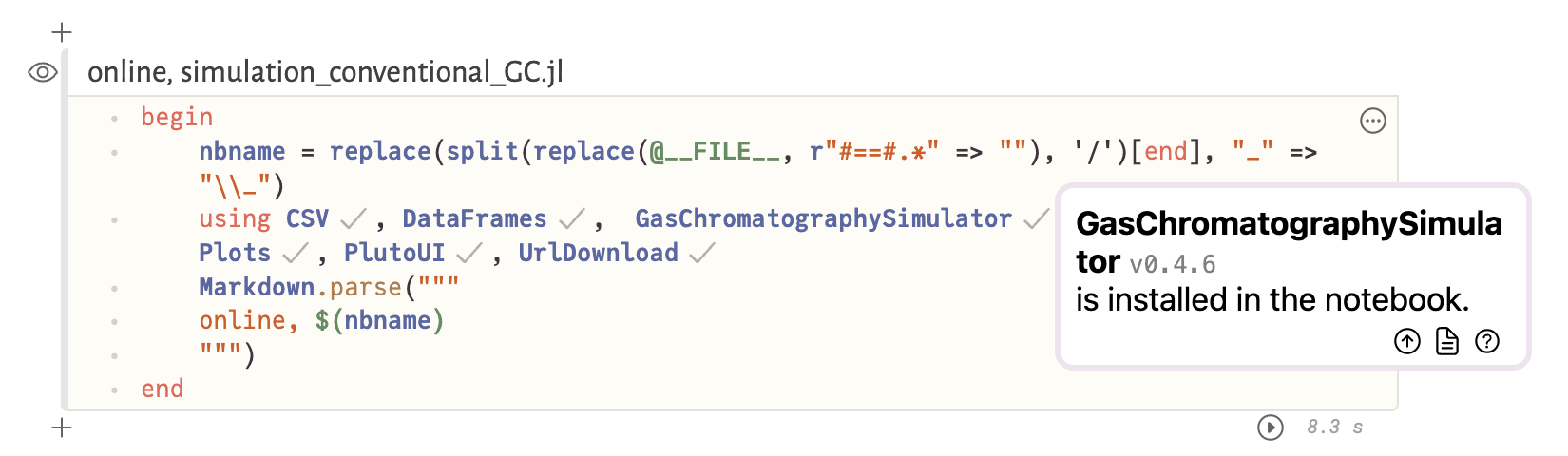The loaded versions of the packages can be checked by clicking on the check marks next to the package name. In this example the latest version 0.4.6 of GasChromatographySimulator.jl was loaded. By clicking on the circle with the upwards arrow a newer version, if available, can be loaded.

Settings

After the header and the title with a short description of the notebook the settings for the simulation follow.

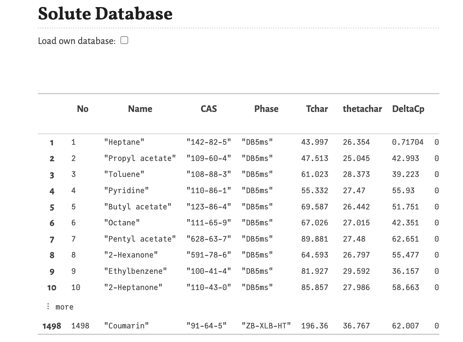
Solute database

Here the database with retention parameters is loaded. As default the database from RetentionData is loaded. The retention parameters are expressed with the three parameter Distribution-centric model by Leonid M. Blumberg.

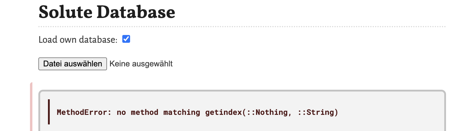
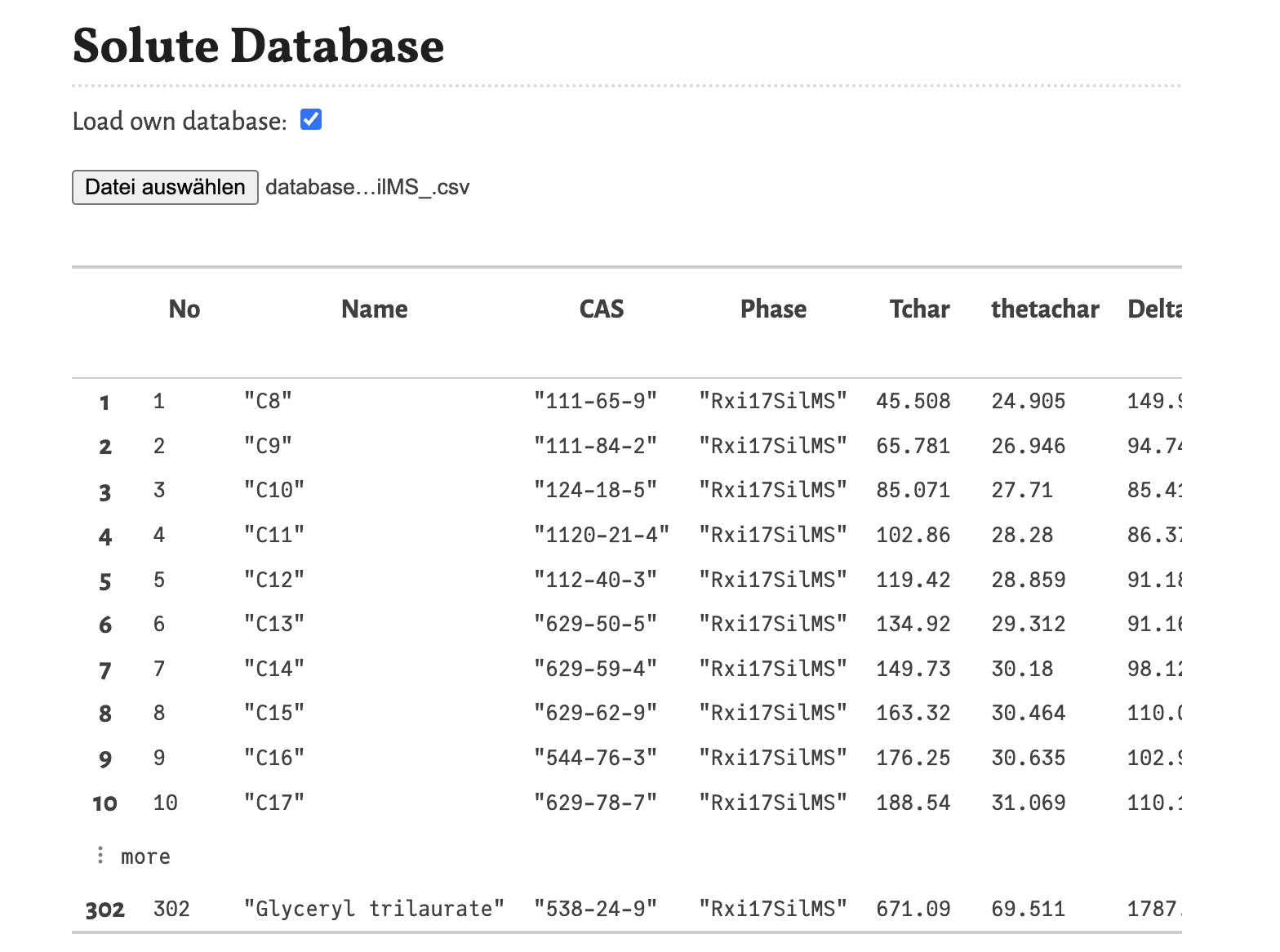
You can load another database by activating the option “Load own database”. In this case a file picker appears, which you can click and than select the file. After activating this option, the following cell reports an error, because no database was selected yet.

The database should be a .csv-file with the following structure:

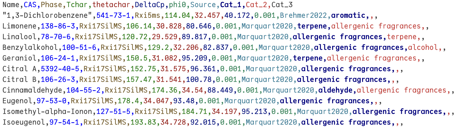
The database has 11 columns containing different information and every row contains the information for one substance. The saved information are:

• Name - Name of the substance. If a name contains a comma, the name has to be placed in quotation marks.
• CAS - CAS number of the substance, this information is used for the estimation of the diffusion coefficient based on the formula and molar mass extracted from a database (ChemicalIdentifiers.jl). If the substance is not found, in this database the diffusion coefficient of n-pentadecane is used as placeholder.
• Phase - Label of the stationary phase for which the retention parameters where estimated. The labels of the database are used for the selection of the stationary phase in the column settings.
• Tchar - The first retention parameter, the characteristic temperature T_char. This is the temperature, where k = 1 (or ln k = 0).
• thetachar - The second retention parameter, the characteristic thermal constant θ_char. It is the is the inverse decreasing slope of ln k(T) at T = T_char.
• DeltaCp - The third retention parameter, the change of isobaric heat capacity ΔC_p. It describes the curvature of ln k(T) for T ≶ T_char.
• phi0 - The dimensionless film thickness (d_f/d) of the stationary phase where the retention parameters where estimated. This information is needed to compensate the retention factor for different film thicknesses.
• Source - Here information about the source of the retention parameters can be stored or other annotations can be made here.
• Cat_1, Cat_2, Cat_3 - Categorical descriptors for the substances. This information is later used for the substance selection.

With a successfully loaded own database the output looks like:

It is also possible to use only two parameters of the Distribution-centric model by setting the third parameter ΔC_p = 0.

Option settings

In this notebook only two option settings can be changed.

These options are:

• viscosity model - Selects the model for the viscosity of the mobile phase as a function of the temperature. Options are Blumberg, a non-linear model from Blumbergs book, and HP, a linear model as used in the HP/Agilent flow calculator.
• control mode - Selects the control mode for the flow. Options are Flow, where the flow through the column is defined and the needed inlet pressure is calculated, and Pressure, where the inlet pressure is selected and the resulting flow through the column is calculated.

To apply the changes of the settings the button Confirm (respectively Senden in the screenshots, depending on the language settings of your operating system) must be clicked. Otherwise the change is not registered.

Column settings

Next are the settings regarding the column, including the selection of the type of the mobile phase.

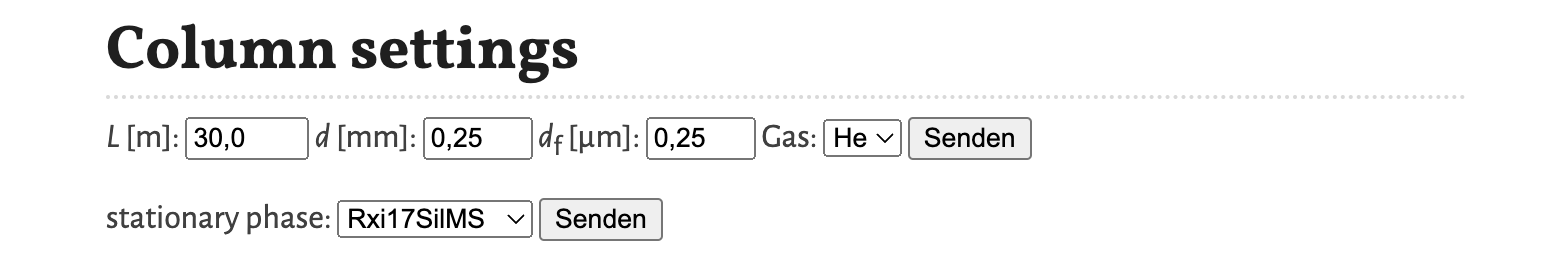
The following settings can be changed:

• L [m] - The length of the column in meters.
• d [mm] - The internal diameter of the column im millimeters.
• df [µm] - The film thickness of the stationary phase in micrometers.
• Gas - The type of the gas of the mobile phase. Available selections are He for helium, H2 for hydrogen and N2 for nitrogen.

Separately, the stationary phase can be selected from stationary phase. The available selection of stationary phases is extracted from the solute database. Changing the database, changes this selection.

Program settings

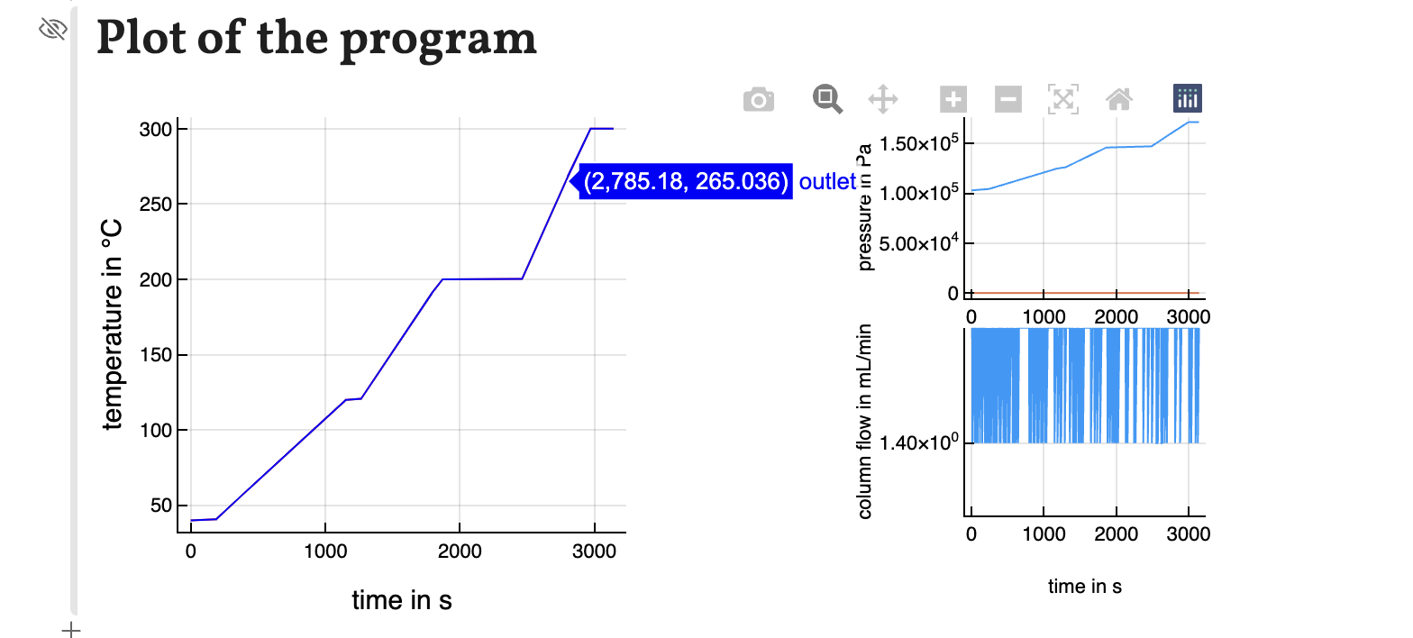
With the program settings the temperature program, the flow respectively the inlet pressure, and the outlet pressure are defined.

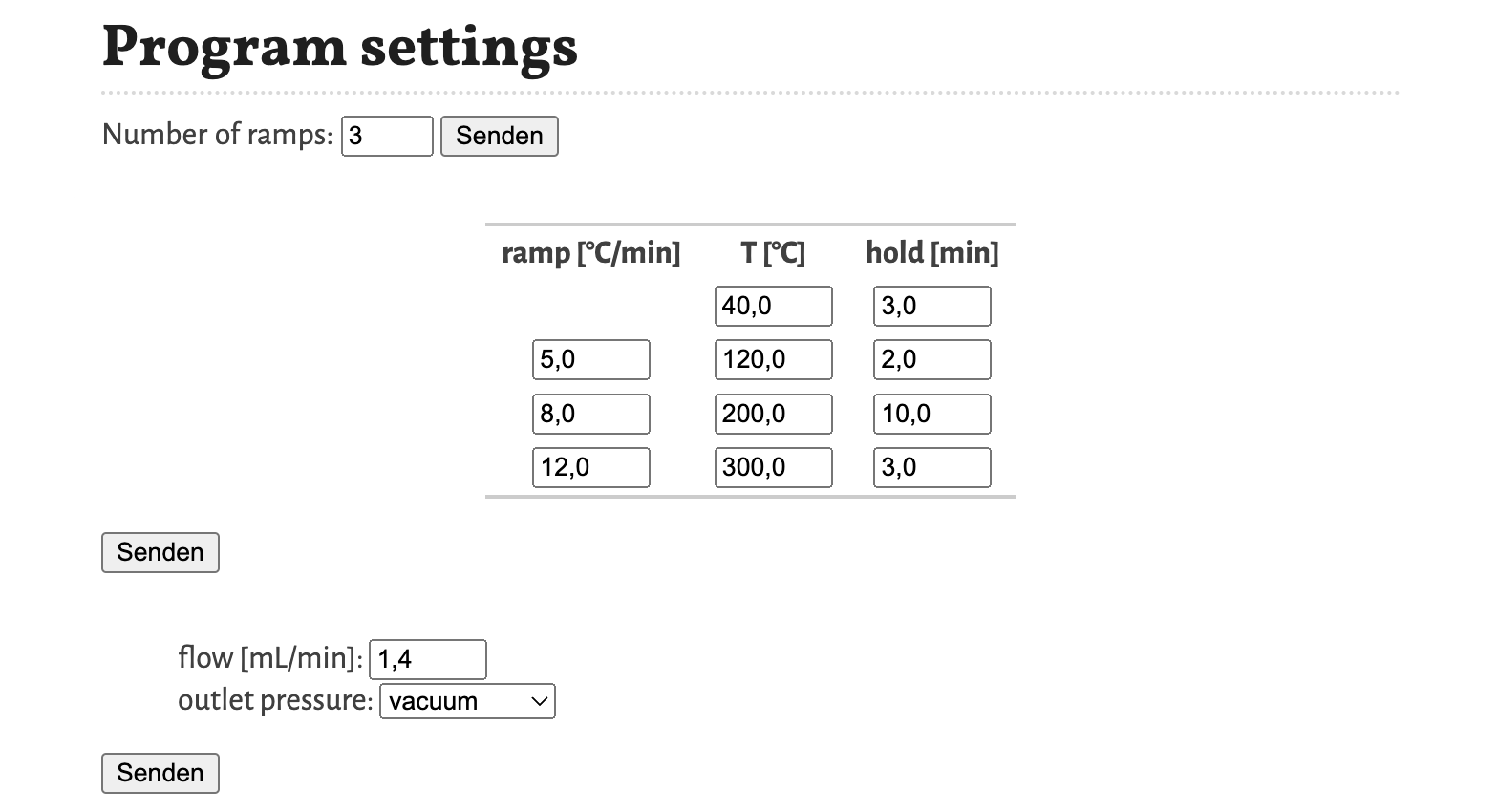
The temperature program is defined first by selecting, how many different heating ramps are used. Based on this selection the table for defining the temperature program is created, with the first column the heating ramp [°C/min], the second column the temperature plateau T [°C] and the third column the hold [min] time of the temperature plateau. In the simulation, the temperature programs continues at the final temperature value until the last substance is eluted.

For the flow program the value of the flow [mL/min] through the column is defined, if the control mode option is set to Flow. If the control mode option is set to Pressure, than the flow program is defined by the inlet pressure [kPa(g)] (gauge pressure). The value of flow respectively inlet pressure is constant throughout the whole program. The outlet pressure can be selected between vacuum (0 kPa) and atmosphere (101.3 kPa).

The temperature, pressure and flow program are plotted as interactive graphs. With the mouse courser the values of the graphs can be shown. The plot can be saved as a .png-file by clicking the camera symbol. It is also possible to zoom into the graph by drawing a rectangle while holding the left mouse button around the area you want to zoom in.

Attention must be given to some links of settings. Changing, for example, the number of ramps changes the temperature program settings and applies the default values.

Substance settings

The final settings section is the selection of the substances which will be used for the simulation of GC. This selection is divided in two steps. With the first step, the category of the substances can be selected. The options for the available categories is extracted from the loaded solute database (from the three columns Cat_1, Cat_2 and Cat_3). In the second step, the the substances can be selected from the list of available substances defined by the selected category and the selected stationary phase.

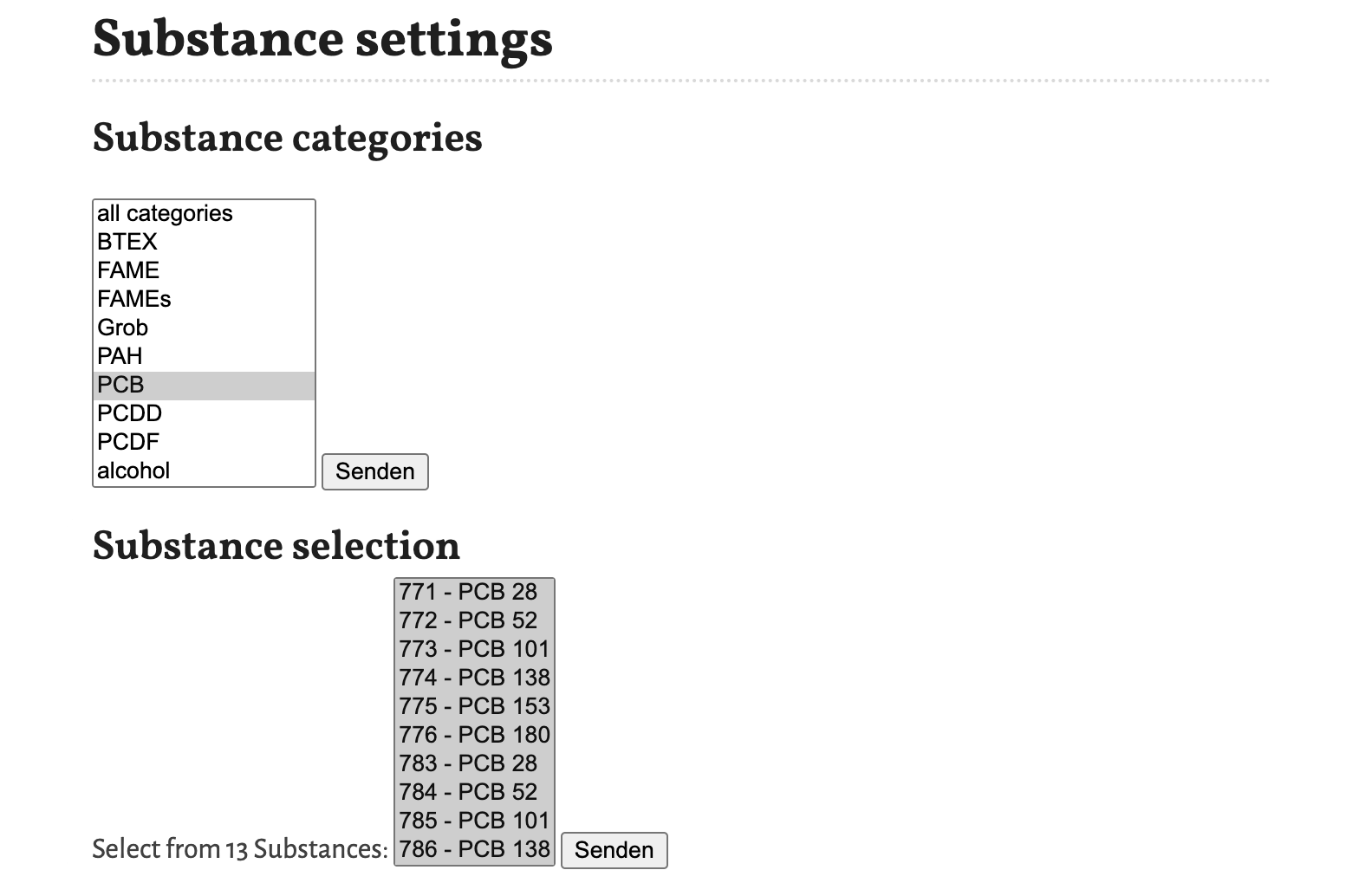
In the shown example PCBs are selected. The number in front of the name is the ID number of the substances in the loaded database. It was introduced to differentiate between multiple entries for the same substance, but with different retention parameters. This is here the case for the substances PCB 28, PCB 52, PCB 101 and PCB 138.

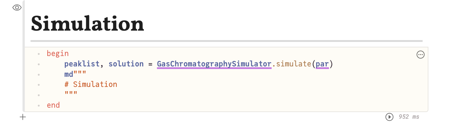
Simulation

Finally we reached the cell in the notebook, where the simulation itself is calculated. In the screenshot below, I made the code visible. It is just this one line. Here the time needed for the simulation of the 13 selected PCB can be seen, which is 1 s. Every time one of the Confirm-buttons in the settings is clicked, the simulation is run.

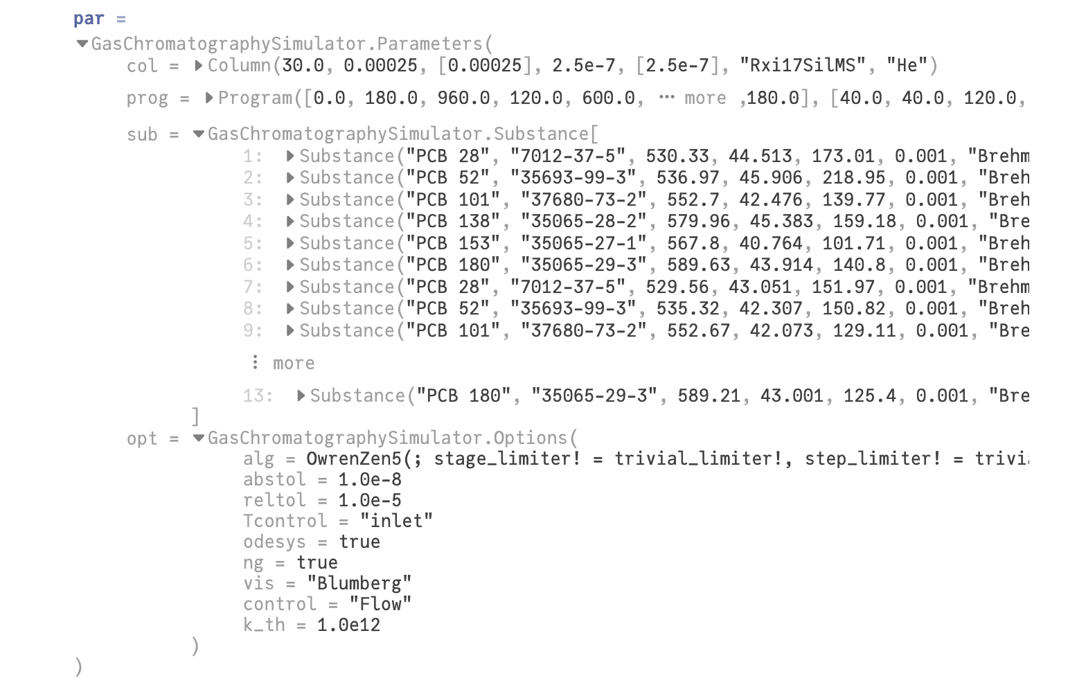
All the settings are collected in the structure GasChromatographySimulator.Parameters labeled here par. This part is hidden at the bottom of the notebook.

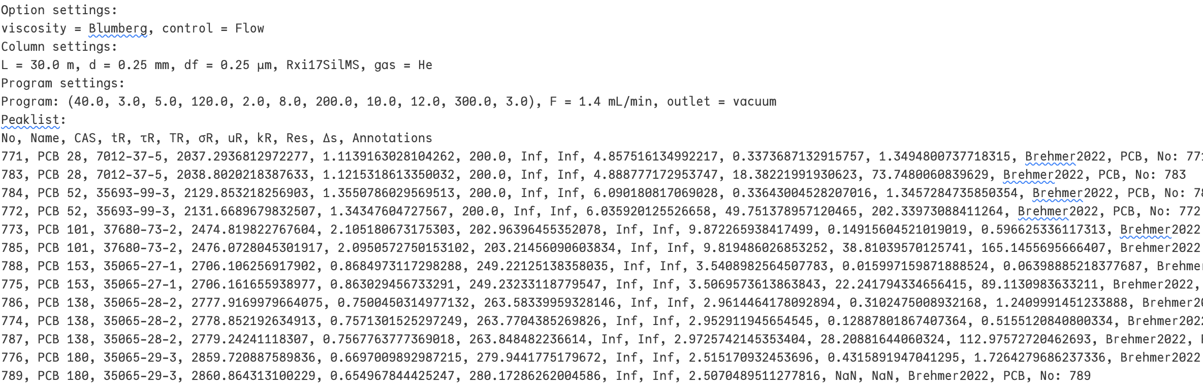
Peaklist

The main result of the simulation is the peaklist. In this table the resulting retention times and peak widths and derived quantities are listed here. The substances are sorted by increasing retention times.

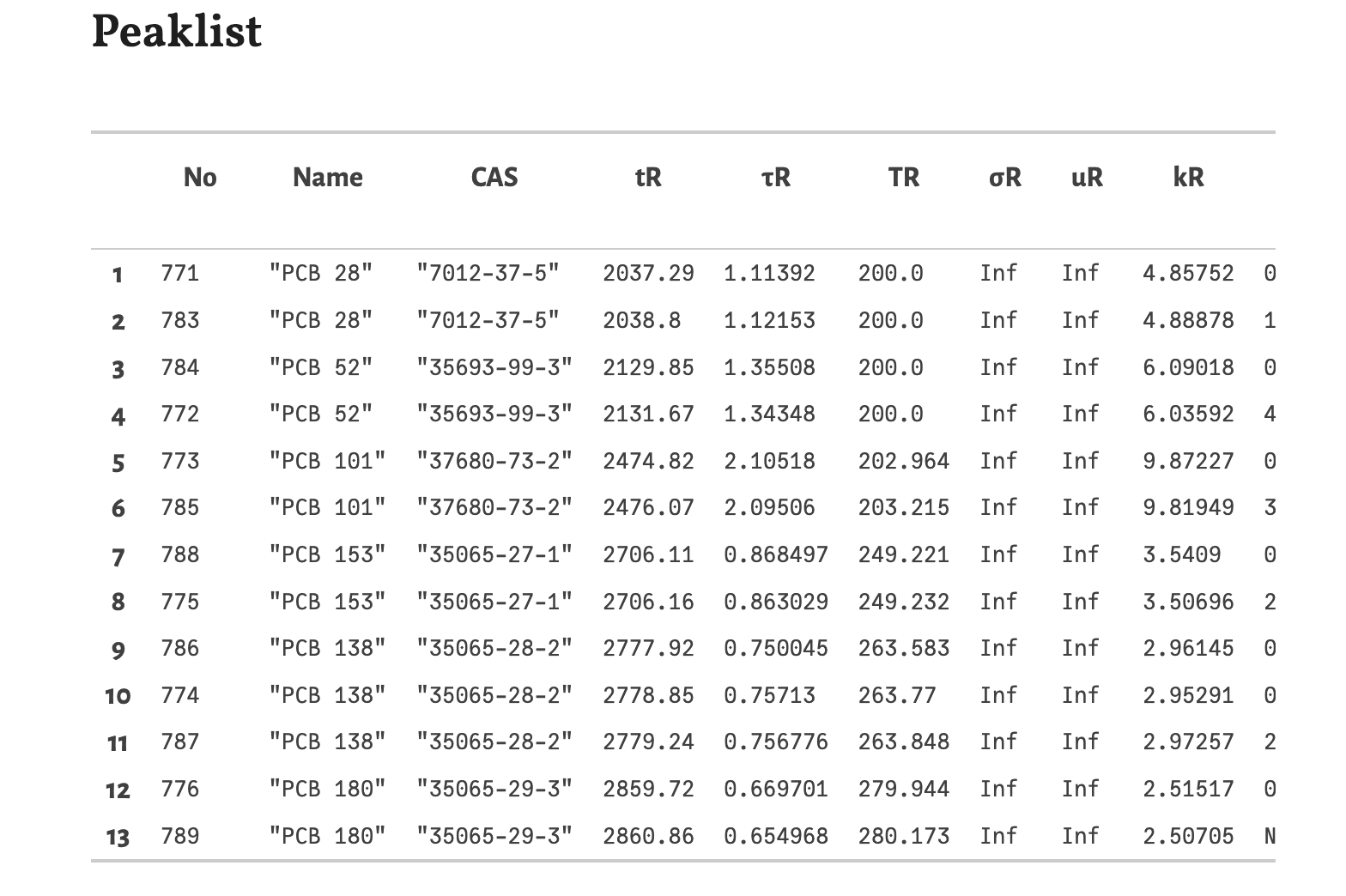
• No - The ID number from the loaded retention database
• Name - The name of the substance.
• CAS - The CAS number of the substance.
• tR - The retention time in seconds.
• τR - The standard deviation of the gaussian peak in seconds. The full width at half maximum (FWHM) can be calculated as 2√2 ln 2 τR.
• TR - The temperature of the GC oven at the retention time in °C.
• σR - The spatial band width at the retention time in meters. Because of the vacuum outlet it is infinite here.
• uR - The linear velocity of the substance at the retention time in meters per seconds. Because of the vacuum outlet it is infinite here.
• kR - The retention factor at the retention time.
• Res - The resolution between neighboring peaks.
• Δs - The separation between neighboring peaks. It is approximately 4 times the resolution.
• Annotations - Collected information, like source and categories of the substances The columns Res, Δs and Annotations are not visible in the screenshot. You have to scroll to the right in the table of the notebook.

  Chromatogram

  Based on the results shown in the peaklist the chromatogram is calculated using gaussian peaks with an area of 1. Therefore the peak hight correlates with the peak width for resolved peaks.

The peaks are numbered by their position in the peak list. As the plot of the program is interactively, the chromatogram is as well. You can zoom in and save is as a .png-file.

Local values

With the last plots local values of time, peak width, temperature, band width and solute velocity can be plotted. This can be used to observe the development of the separation during the migration of the substances through the column.

Export results

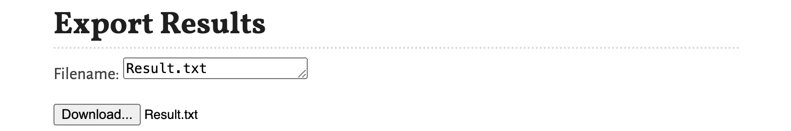
Finally, we can export the results of the simulation in the form of the peaklist including the settings of the simulation. With Filename the name of the exported file can be changed. By clicking the Download button the result is downloaded as the named file into the standard download folder.

Additional notes

As shown in the previous tutorial you can move the cells to other positions in the notebook. This comes in handy, if you want to change some parameters and observe the change in the chromatogram directly as shown here for the variation of the column diameter:

This concludes this tutorial. In the next tutorial I will show, how the notebook estimate_retention_parameters.jl can be used to calculate retention parameters from a small number of GC measurements with different programs.

Please leave a comment if you have more questions about the simulator.